Understanding Focal Loss —A Quick Read
Summary
Focal Loss implications on solving the class imbalance problem
Table of Contents
Yes, you might have got an idea of what I will be discussing in this blog ;p. But before going to the main topic, I want to implant some of the prerequisite points.
- In the case of object detection
- Positive examples: Target Class or foreground information such as ground-truths.
- Negative examples: Non-Target Class or background information such as anchors whose IoU with ground-truths is less than a given threshold.
- Easy positives/negatives: Samples classified as positive/negative examples.
- Hard positives/negatives: Samples misclassified as negative/positive examples.
2. Class Imbalance Problem
- This is observed when information related to one class in a dataset or mini-batches used in training is over-represented than the other classes.
- Training a network on an imbalanced dataset will make the network biased towards learning more representations of the data-dominated class and other classes will be underlooked.
- In the case of Object Detection, two confidence values are predicted. One is Objectness score(Whether an object is present in a box or not) and the other is Class score(To which class detected object belong to).
- So it becomes important to maintain a balanced state between foreground-background and foreground-foreground classes while training. If not handled, former creates a box confidence errors(Whether or not an object is present)and the latter creates class confidence errors(If an object is present in the box, then which class does it represent) during training.
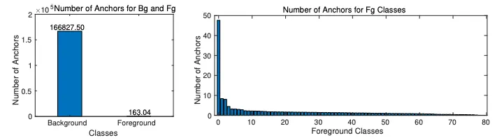
- Two-Stage Detectors have region proposal extractors, that give out many proposals(both. positive and negative) which are further mitigated by some of the sampling techniques mentioned in [1] such as Online Hard Example Mining and IoU/Objectness Thresholding.
- On the contrary, One-Shot detectors do not contain region proposal architecture. They directly undergo global regression/classification from feature maps and generate a fixed amount of anchors per location. It becomes somewhat difficult to apply these sampling heuristics to get rid of unwanted negative samples.
- Even, if applied, the network then also becomes biased towards learning background information which is of no use. This is illustrated below in a given snippet.
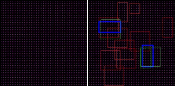
| Setting | Value | Note |
|---|---|---|
| Image size | (400, 400) | Image input dimensions |
| Output feature map size | (50, 50) | Stride of 8 |
| Anchor boxes | (45, 90), (90, 90), (90, 45) | |
| Ground truth | [50, 100, 150, 150], [250, 210, 300, 310] |
Configuration set for the YOLO network, with IoU thresholding applied.
| Count | |
|---|---|
| 1. Total anchors present at each location | 7500 (50 × 50 × 3) |
| 2. After removing invalid anchors, total remaining anchors | 5301 |
| 3. Total number of Positive RoIs (IoU > 0.5) | 5259 |
| 4. Total number of Negative RoIs (IoU <= 0.5) | 42 |
- As seen from the above Fig. 1 and snippet, there is a vast difference between positive and negative samples, stating a proper imbalance between Foreground and Background in these kinds of detectors(YOLOv3[2] have 3 anchors per location on a feature map at a particular scale).
- Some of the challenges which are been faced in training due to imbalance in a dataset are(stated in [5]):-
- Training becomes inefficient as most of the samples are easy negatives which contribute no useful signal. This kind of bias makes difficult for a network to learn rich semantic relationships from the images.
- Cumulative easy negatives loss overwhelms the total loss, which degenerates the model.
To solve the above problems Facebook A.I came up with a new modified approach by adding a weighting to cross-entropy loss. Let’s now get straight into the topic for which this article is meant for. Brush Up ;).
1. Focal Loss
What is a focal loss in laymen’s term?
Let’s consider a scenario of a soccer match. You are seeing your favorite rivalry of Real Madrid vs Barcelona on television. The stadium is fully packed with the audience chanting for their respective teams with a total of 70,000 people. Suddenly Real Madrid scores and whole stadium bursts will the chants of “Goaalll..!!”. No one can hear anything but chants, chants, and chants. 3 commentators are analyzing the match that these telecast reporters want to show on the TV. So what they do to? They give more importance to the commentary and give less weight to the chants so that people watching on television can listen to the commentary and live match analysis. Yes, you will hear the chants while watching but, commentary voice will get more amplified. Remember this analogical example for now.We will see how this example relates to Focal Loss
Let’s devise the equations of Focal Loss step-by-step:
- Let's read Eq. 1 case by case. Cross-entropy charges −log(p) when the box is foreground (y = 1) and −log(1 − p) when it is background. Either way, the bill is small when the probability given to the correct class is high and large when it is low.
- Numbers are always satisfying to justify something. Take a foreground box: p = 0.9 costs −log(0.9) = 0.105, while p = 0.1 costs −log(0.1) = 2.303. Being wrong is 22× more expensive than being right, which is exactly what we want so far.
- Modifying the above loss function in simplistic terms, we get:-
- Two cases are one case too many, so let's fold them into a single number. p_t is simply the probability the model gave to whatever the true class was: p if the label is foreground, 1 − p if it is background.
- Say the model outputs p = 0.8. If the box is foreground, p_t = 0.8 (easy, well classified). If the same box is actually background, p_t = 1 − 0.8 = 0.2 (hard, misclassified). So a large p_t means an easy example and a small p_t means a hard one.
- Slide p in the figure below and read off p_t for both labels. The two lines cross at p = 0.5, where the model is just guessing.
- With p_t in hand, both branches of Eq. 1 collapse into one line: CE(p_t) = −log(p_t). This is the loss Focal Loss is going to modify.
- Now the catch. Even an easy example with p_t = 0.9 still costs −log(0.9) = 0.105. That looks harmless until you remember there are tens of thousands of such easy negatives per image: 10,000 of them add up to 10,000 × 0.105 = 1,050, while one hard positive at p_t = 0.1 contributes only 2.3. The chants drown the commentary.
- α term is added to the above Eq 3. to handle the class imbalance problem. It is a hyperparameter that can be used with the CE loss function for cross-validation. α_t is a weighted term whose value is α for positive(foreground) class and 1-α for negative(background) class.
- α_t is a per-class weight, defined exactly the same way as p_t: α for the foreground class and 1 − α for the background. It is the standard remedy for class imbalance, giving the rare class more say per example.
- With α = 0.25, every foreground example is weighted 0.25 and every background example 1 − 0.25 = 0.75.
- Eq. 5 is α-balanced cross-entropy: the loss of each example is scaled by its class weight α_t. This rebalances positives against negatives.
- But look at what it does to two negatives. With α = 0.25, an easy negative at p_t = 0.9 costs 0.75 × 0.105 = 0.079 and a hard negative at p_t = 0.1 costs 0.75 × 2.303 = 1.727. Both got the same 0.75; the weight cannot tell easy from hard. That is why α alone is not enough.
- Slide α in the figure below: the foreground curve rises and the background curve falls together, but neither curve changes shape.
- Eq 5. only handles and controls the weight of positive and negative samples, but it doesn’t take into consideration easy and hard samples. So finally, Focal Loss was designed in such a way that it handles both the mentioned conditions. Two forms of Focal Loss are given below.
Non-alpha form
- Here it is, the Focal Loss. Cross-entropy is multiplied by a modulating factor (1 − p_t)^γ. When an example is already well classified (p_t close to 1) the factor is close to 0 and the loss is almost switched off. When it is misclassified (p_t small) the factor is close to 1 and the loss is left as it is.
- γ is the focusing parameter; it sets how sharp the switch is. γ = 0 gives back plain cross-entropy.
- Numbers again. At γ = 2, an example with p_t = 0.9 keeps (1 − 0.9)² = 0.01 of its loss, i.e. 1%: 0.01 × 0.105 = 0.001, 100× smaller than cross-entropy. One with p_t = 0.1 keeps (1 − 0.1)² = 0.81, i.e. 81%. The commentary is amplified, the chants are turned down.
- Slide γ in the figure below and watch the factor against p_t: the higher the γ, the earlier the curve drops to zero.
Alpha Form
- This is the form used in practice: the modulating factor and the class weight α_t together. The paper found γ = 2 with α = 0.25 to work best.
- Notice α is below 0.5, which looks backwards for a rare foreground class. The reason: once γ has down-weighted the easy negatives, the positives no longer need as much help. Multiply it out for γ = 2, α = 0.25: an easy negative at p_t = 0.9 costs 0.75 × 0.01 × 0.105 = 0.0008, a hard positive at p_t = 0.1 costs 0.25 × 0.81 × 2.303 = 0.466, about 590× more.
- The interactive graph further down compares this loss with cross-entropy as γ and α change.
Visualization and Results of Focal Loss
NOTE: In the case of class imbalance(BG >> FG)
— hard(Misclassified) examples are False negatives(Predicted as background, query box is foreground)
— easy(Correctly Classified) examples are True negatives(Predicted as background, query box is background)
Now recall the analogy stated earlier and compare it with Focal Loss. All the hard(or misclassified — false negatives) samples are given more weight while learning than easy(correctly classified — true negatives) examples. So, even if the imbalance problem is prevalent, this condition is taken care of by Eq. 8.
Final Focal Loss(Alpha Form)
- Eq. 8 is the same loss written out for the two labels, so you can implement it straight from p. For y = 1 the factor is (1 − p)^γ and the weight α; for y = 0 the factor is p^γ and the weight 1 − α.
- Take the same prediction p = 0.9 with γ = 4 and α = 0.25. If the box is foreground: 0.25 × 0.1⁴ × 0.105 = 0.0000026, practically nothing. If the box is background, p = 0.9 is a confident miss: 0.75 × 0.9⁴ × 2.303 = 1.133. Same p, two labels, a loss that differs by five orders of magnitude.
- The two graphs below plot exactly these two branches; the sliders change γ and α in both at once.
- Below given are the graphs of the Cross-Entropy and Focal Loss(alpha form) for given α_t =0.25 and γ = 4 for given input in the range [0,1].
- As we can see from the above-given graphs, it is visible how the loss is propagated for easy examples. For correctly classified examples, the cross-entropy loss at p=0.5 is 0.62 while in the case of 0.00034. Focal Loss decreases the slope of the function which helps in backpropagating(or weighing down) the loss.
- α and γ are hyperparameters that can be tweaked for further calibration. γ can also be said as a relaxation parameter in laymen’s terms.
- More the value of γ, more importance will be given to misclassified examples and very less loss will be propagated from easy examples. According to the study mentioned in [5], γ=2 gives the best results.
- Numbers are always satisfying to justify something. So let’s play with some numbers and focal loss. Below given snippet proves that the easy examples are given less weight than misclassified examples.
| Loss | For positives | For negatives |
|---|---|---|
| Cross-Entropy | -log(x) | -log(1 - x) |
| Focal Loss (Alpha Form), alpha = 0.25, gamma = 2 | -alpha · (1 - x)gamma · log(x) | -(1 - alpha) · xgamma · log(1 - x) |
Focal and Cross-Entropy Loss comparison for proving down-weighting of easy examples.
| Case | x | Cross-Entropy Loss | Focal Loss | CE/FE |
|---|---|---|---|---|
| 1. Easy example (correctly classified, y = 1, x ~ 1) | 0.9 | 0.045 | 0.000125 | 360 |
| 2. Hard example (misclassified, y = 1, x ~ 0) | 0.1 | 1 | 0.2025 | 40 |
- From the above snippet, the CE/FE ratio in case of an easy classification is 360 and in case of a hard classification, it’s just 40 which justifies the stated premise.
2. Conclusion
Focal loss is used to address the issue of the class imbalance problem. A modulation term applied to the Cross-Entropy loss function, make it efficient and easy to learn for hard examples which were prevailing in One-Shot Object Detectors.
If you have managed to reach here, then I believe you are a part of an elite group who have a thorough understanding to get started in the captivating problem of class imbalance and focal loss.
Please feel free to share your thoughts and ideas in the comment section below.
If you think that article was helpful, please do share it and also clap(s) would hurt no one.
3. References
[2] YOLOv3: An Incremental Improvement, Joseph Redmon, Ali Farhadi
4. Connections
What this page builds on, cites or links to, and what points back at it. A plain box is a “builds on”; “cited” and “linked in the text” are the lighter links. Hover a box for a preview.
Related
- Read · this builds on it
- Paper · builds on this
- Paper · builds on this
- Paper · builds on this
- Project · same tag: Class imbalance
- Paper · same tag: Loss functions, Object detection
Go deeper
-
Start withRead
-
You are hereUnderstanding Focal Loss —A Quick ReadPaper
-
ThenPaper
-
Paper
-
Paper
-
Paper
-
Paper
-
Read
-
Paper
-
Paper
-
Read
-
Paper
-
Paper
-
Paper
-
Paper
-
Paper
Go broader
- Sits underObject detection › Focal loss
- Its tags on the map
- Also under these tagsYOLOv4 — Version 1: Bag of FreebiesLoss functions, Object detectionTriplet Loss Demystified in 5 minsLoss functionsIn defense of triplet loss for person re-identificationLoss functionsBenchmark Datasets: Gas-station for CVObject detectionSynthetic Bounding Box GenerationObject detection
- Ask the mapWhat connects Focal loss and …type the other page's name; the map answers with the chain of links between them