YOLOv4 — Version 2: Bag of Specials
- 1YOLOv4 — Version 0: Introduction
- 2YOLOv4 — Version 1: Bag of Freebies
- 3YOLOv4 — Version 2: Bag of Specials
- 4YOLOv4 — Version 3: Proposed Workflow
- 5YOLOv4 — Version 4: Final Verdict
Summary
An Introductory Guide on the Fundamentals and Algorithmic Flows of YOLOv4 Object Detector
Table of Contents
- 0. What is Bag of Specials?2
- 1. Mish Activation2
- 2. CSP(Cross Stage Partial Connections)2
- 3. FCN-Spatial Pyramid Pooling2
- 4. Spatial Attention Module(SAM)2
- 5. Path Aggregation Networks(PANet)2
- 6. DIoU NMS⁹2
- 8. References2
- 9. Connections2
Welcome to the mini-series on YOLOv4. This article will be addressing all the components authors have presented in the part Bag of Specials. So, breathe in, breathe out, and enjoy learning.
YOLOv4 — Version 0: Introduction
YOLOv4 — Version 1: Bag of Freebies
YOLOv4 — Version 2: Bag of Specials
YOLOv4 — Version 3: Proposed Workflow
YOLOv4 — Version 4: Final Verdict
This article will specifically target all the questions about the different methods present in this Special Bag.
Once progressed to the end, you will get a very demanding understanding of the working and advantages of the same.
All the attributes will be explained in an independent manner so that you can get a good taste of these ingredients before adding into your final recipe ;).
0. What is Bag of Specials?
- As mentioned by the authors:-
Bag of Specials contains different plugins and the post-processing modules that only increase the inference cost by a small amount but can drastically improve the accuracy of the object detector.
- In general, these methods or Bag of Specials can be considered as an add-on for any object detectors present right now to make them more accurate on benchmark datasets.
- Yeah, the selection of the methods may vary with the different architectures of Object Detectors, but the final goal of refining the detector results will be achieved.
- There are many different modules present, but as right now we are focusing on YOLOv4, we will only discuss these selective methods shown in Fig. 1 in a robust manner by answering whats and whys of the same.
1. Mish Activation
1.1 What are the problems faced by recent Activation Functions?
- ReLU(Rectified Linear Unit) is one of the most famous activation functions present in SOTA Convolutional Neural Networks. It’s easy differentiability and zero cost are the biggest advantages that make them the first choice.
- As shown in Fig. 2 ReLU is a function ramped at 0. Differentiation of this function for negative values is 0 hindering the gradient descent method as 40% of network neurons will not get updated. So Leaky ReLU was invented to solve the problems of dead neurons or dying ReLU but did not perform up to the mark. This makes a huge impact on training if a neuron always outputs negative values.
1.2 Slow but effective: Entry of Mish.
- Mish² is a novel activation function similar to Swish³ and is defined as.
Fig. 3 Above) graph of Mish Function. Below). Equation of Mish Function.
- Mish multiplies the input by the hyperbolic tangent of softplus(x) = ln(1 + eˣ). Let's walk it through.
- For large positive x, tanh(softplus(x)) → 1 so Mish ≈ x, like ReLU: at x = 3, softplus = ln(1 + e³) = 3.05, tanh(3.05) = 0.996, and Mish = 2.99.
- For negative x it is small but not zero, and it dips slightly below zero before returning to it: at x = −1.2 Mish is −0.31, at x = −5 it is −0.03. So the gradient never dies and the function is smooth everywhere. The graph above traces it; move x along the curve and watch the dip.
- Properties of Mish Activation Function are:-
— Non-monotonic function: Preserves negative values, that stabilize the network gradient flow and unlike ReLU, and almost solving Dying ReLU problem and helps to learn more expressive features.
— Unboundedness and Bounded Below: Former helps to remove the saturation problem of the output neurons and the latter helps in better regularization of networks.
— Infinite Order of Continuity: Unbiased towards initialization of weights and learning rate due to the smoothness of a function helping for the better generalizations.
![Fig 4. More transient jumps are seen in the ReLU output landscape as compared to Mish. [Source: [2]].](/images/reads/yolov4-bag-of-specials/06.webp)
— High compute function but increases accuracy: Although being high-cost function, it has proven itself better in deep layers in comparison to ReLU.
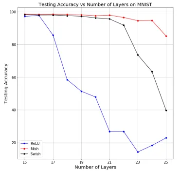
— Scalar Gating: Scalar Gating is an important property of this function and so it becomes logical and can easily replace the pointwise functions like ReLU.
Using Mish as an activation function in YOLOv4 showed decent amount of accuracy gains. Mish Activation + CSPDarknet53 combo gave the best results in the ablation study mentioned in the paper.
Increased some computational cost, but showed good refinement of the detector results. Bag of Specials definition hence proved..!!
| Model (with optimal setting) | Size | AP | AP50 | AP75 |
|---|---|---|---|---|
| CSPResNeXt50-PANet-SPP | 512x512 | 42.4 | 64.4 | 45.9 |
| CSPResNeXt50-PANet-SPP (BoF-backbone) | 512x512 | 42.3 | 64.3 | 45.7 |
| CSPResNeXt50-PANet-SPP (BoF-backbone + Mish) | 512x512 | 42.3 | 64.2 | 45.8 |
| CSPDarknet53-PANet-SPP (BoF-backbone) | 512x512 | 42.4 | 64.5 | 46.0 |
| CSPDarknet53-PANet-SPP (BoF-backbone + Mish) | 512x512 | 43.0 | 64.9 | 46.5 |
Fig 6. Results using Mish in Backbone.
2. CSP(Cross Stage Partial Connections)
2.1 Prerequisite: What is DenseNet⁴?
- DenseNet is a different architectural design that can be used as a backbone for different detection and classification tasks.
- As we can see from the above figure, DenseNet contains chains of Dense and Transition Blocks.
- DenseNet leverages the idea of ResNet i.e information from the previous layer is added to the output of the present layer, also known as skip connections.
- Unlike ResBlock, each layer in DenseBlock is connected to every other layer and instead of the channel-wise output addition of feature maps, there is a channel-wise concatenation as shown in the below-given figure. After every dense layer, channels are concatenated instead of doing element-wise addition.
- Here, Dense Block comprises of chains of Dense Layers. These Dense Layers follows an architecture of a simple Conv+BN+ReLU combo with an output filter size of growth rate k. Growth Rate is used to control the number of final output channels of a dense block. If Dense Block contains N dense layer, the final output number of channels will be N*k + baselayer filters(16 as shown in Fig. 8).
- Height and Width of a feature map remain constant in one dense block. As CNNs are downsampled to get enriched features and reducing computational cost: this work is done by a Transition Block. It simply downsamples the output of a dense block and also reducing the number of channels of that particular feature map.
2.2 What is the problem with DenseNet alike architecture?
- In a dense block, layer k does not see only the previous layer. Its input is the concatenation of the block's input x₀ and every output x₁ … x_{k−1} produced so far, and w_k is the convolution applied to that stack.
- Each layer therefore reads the same early channels again, and the width of its input grows linearly with k. With 16 base channels and a growth rate of 16, six layers read 16, 32, 48, 64, 80 and 96 channels, 336 channel-reads in total, and x₀ is read six times over.
- The figure below counts the channels each layer reads; raise the growth rate or the number of layers and the bars climb. The early channels are counted once per layer, which is the duplication CSP sets out to remove.
Fig. 9 (Left) Forward Pass in each dense block. (Right) Gradient Flow in a dense block. (Source: [4]).
- Now the backward pass. The weight update for layer k depends on its own gradient and, through the concatenation, on the gradients g₀ … g_{k−1} flowing from every earlier layer.
- The boxed terms are the ones that appear in every row: g₀ shows up in all k updates, g₁ in k − 1 of them, and so on. For a block of 6 layers that is 6 + 5 + 4 + 3 + 2 + 1 = 21 gradient terms to update 6 layers. The same gradient information is used to update many different layers, so much of the backward pass is spent on duplicated signal.
- As shown in Fig. 9, input to the kth dense block will be the concatenated output of previous k-1 dense layers. While doing a gradient descent, all the dense layer weights will be updated with a copy of the same gradients as shown in Fig. 9(Left). This results in inefficient optimizations of a network and will have a redundant inference cost.
2.3 Entry of Cross Stage Partial Connections⁵
- To solve the problem of replicated gradients, input to a dense block is divided into two parts. One is used directly into the concatenation with the final output of the DB+TB chain and the other is used as an input in the dense block as shown in Fig. 10.
- Advantages of CSP Connections are:-
- Increasing the gradient flow paths that help in removing the replicated updates of the weights in DenseBlock.
- Breaking a base layer into two parts helps to decrease the number of multiplications in Dense Block, which further helps in increasing inference speed.
- CSP design can be used in any backbone of network architecture. It has proved to increase a decent amount of accuracy in almost the same inference time.
In YOLOv4, this design is integrated with the original Darknet53 model of YOLOv3. CSPDarknet53 with some other tuning parameters have proved to give the best results. We will see this in our 5th part of this series.
3. FCN-Spatial Pyramid Pooling
3.1 What is Spatial Pyramid Pooling⁶?
![Fig. 11: Making of 1-d Vector from SPP operation(Source[6]).](/images/reads/yolov4-bag-of-specials/15.webp)
- During classification tasks, the output feature map is flattened and directed to the FC layer for further softmax operation. However, to use the FC layer, we have to fix the size of an input image while training that hinders to detect objects at different scales and object aspect ratios.
- To solve this issue, the final output feature map undergoes channel-wise pooling for different sizes of spatial bins. If input feature map dimensions are 512X100X100(CXHXW) and spatial bins are 1X1, 2X2, 4X4, then SPP generates 512, 4*512, 16*512 1-D vectors which are then concatenated to feed into FC layer.
- Each 2-D feature map is averaged over a total of HXW values to generate value in that spatial bin. NXN window size in SPP means to divide an image into equal NXN spatial bins as shown in Fig. 11.
3.2 How to leverage SPP in Fully Convolutional Networks?
- As seen in 3.1 conventional SPP generated 1-D output, which cannot be used in FCNs like YOLO. So how can we solve this issue?
- Here before passing the output feature map to YOLO-Head, it is passed to different convolutional blocks of kernel size 1x1, 3x3, 9x9, and 13x13 to increase the receptive field and capture different object patterns at different scales. These are concatenated and then passed to the final prediction stage or YOLO Head.
In YOLOv4, SPP is used as an extra module to increase the receptive field. Backbone is comprised CSPDarknet53. So this module is used after the ((DB+TB)+TB) blocks i.e after partial connections as discussed in section 2.
4. Spatial Attention Module(SAM)
4.1 What is an Attention Module
- Attention modules are recently used in Convolutional Neural Nets to make network focus not on the whole but specifically on the objects present in an image.
- These modules help to solve the where and what questions by telling a network to give more weight on the contextual information around an object and which features are important respectively.
- Squeeze and Excitation and Spatial Attention Modules are channel-wise and spatial-wise attention layers respectively that are widely used in CNNs.
4.2 How Pointwise Attention Module is coupled in a network — SAM⁷
- As shown in the figure, YOLOv4 went with pointwise convolution instead of converting the feature map by applying average and max pooling.
- Here sigmoid activation function is used after the convolutional block. This helps to magnify all the object’s contextual information. Values that are not playing any role in the detection/classification task will be down-weighted.
- This refined feature map is multiplied element-wise to get an attention output feature map(dark blue color).
YOLOv4 uses pointwise attention in their architecture design. This attention mechanism can be easily in between ResNet blocks present in CSPDarkNet53. Pointwise attention mechanism increases computational cost by 0.1%.
5. Path Aggregation Networks(PANet)
- Path Aggregation Networks⁸ is one version up of Feature Pyramid Networks.
- FPNs are very versatile and till now many architectures are using it for its transferring and combinations of local(low-level) and global(high-level) features. It helps to combine the rich semantic features from upper levels and good localization features from lower levels which are then used as final maps for prediction.
- PANs work similarly to FPNs, but they added a bottom-up augmentation path as shown in Fig. 14(Below) so that strong texture responses from low levels can directly be fused with semantically rich responses present in N5 using a shortcut path(Only ~10 layers are present between them).
- Here also in PANNet, all the output feature maps from last bottom-up pyramid are fused using ROIAlign and FC Layers so that, all the variabilities of feature maps can be used for the prediction which is not in case of FPNs as at the time of prediction only one feature map based on the scale of an object is used and all the other feature maps will useless.
In YOLOv4, Modified PAN Neck is used for feature aggregation as shown in Fig. 14(Above). Instead of addition, concatenation approach is used between every bottom-up layer. This helps in conserving the missed out or FPN+Bottom Up features at the same time. Of course, this will increase the computational power, but Bag of Specials it is… Bound to happen ;).
6. DIoU NMS⁹
NMS is used to reduce redundant boxes based on IoU metric system. However by using this method, many times two overlapping distinct boxes are suppressed to one box, due to the confidence threshold.
To solve this issue the paper suggests using DIoU-distance. Along with overlap areas of boxes the center points of boxes are equally important. For the predicted box M with the highest score, the DIoU-NMS can be implemented as:
Fig. 14:Source: [Link]
- DIoU-NMS. For a candidate box B_i and the box M already kept, ordinary NMS drops B_i when their IoU exceeds ε.
- DIoU-NMS first subtracts R_DIoU, the squared distance between the two centres divided by the squared diagonal of the smallest box enclosing both, and only then compares with ε.
- Numbers: two boxes with IoU = 0.6 and ε = 0.5. Plain NMS kills the second one. If their centres are 40 px apart inside an enclosing box with a 100 px diagonal, R_DIoU = (40/100)² = 0.16, so 0.6 − 0.16 = 0.44 < 0.5 and B_i survives. Two boxes that overlap heavily but have centres far apart are probably two neighbouring objects, and the penalty lets the second one live.
- Slide the candidate box across the kept one in the figure below and compare what plain NMS and DIoU-NMS decide at the same overlap.
s_i: the classification score.
ε: the NMS threshold.
The box B_i is removed by simultaneously considering the IoU and the distance between central points of two boxes. If the centers are distant enough then they are considered as 2 different objects.
This ends the long explanation of Bag of Specials used in YOLOv4. I hope you have got a good amount of ideas by these independent modules and their relevance with YOLOv4 architectural designs.
Stay tuned to for the detailed explanatory versions of this beautiful research.
Next Article: YOLOv4 — Version 3: Proposed Algorithm.
YOLOv4 — Version 3: Proposed Workflow
Please check out other parts of our entire series on Yolov4 on our page VisionWizard.
It looks like you have a real interest in quality research work if you have reached till here. If you like our content and want more of it, please follow our page VisionWizard.
Do clap if you have learned something interesting and useful. It would motivate us to curate more quality content for you guys.
Thanks for your time :)
8. References
[1] YOLOv4
[2] Mish Activation
[3] Swish Activation
[4] DenseNet
[5] CSPNet
[9] DIoU-NMS
9. Connections
What this page builds on, cites or links to, and what points back at it. A plain box is a “builds on”; “cited” and “linked in the text” are the lighter links. Hover a box for a preview.
Related
- Paper · builds on this (next in the series)
- Paper · explains a paper this cites
- Paper · this builds on it (earlier in the series)
- Paper · same series: YOLOv4
- Paper · same series: YOLOv4
- Paper · builds on this
Go deeper
-
Start withRead
-
Paper
-
Paper
-
You are hereYOLOv4 — Version 2: Bag of SpecialsPaper
-
ThenPaper
-
Read
-
Read
-
Paper
-
Read
-
Paper
-
Paper
-
Paper
-
Paper
-
Read
-
Paper
-
Paper
-
Read
-
Paper
-
Paper
-
Paper
-
Paper
-
Paper
-
Paper
-
Paper
-
Paper
-
Paper
-
Paper
-
Paper
-
Paper
Go broader
- Sits under
- SeriesYOLOv4part 3 of 5 · start from the first part
- Its tags on the map
- Also under these tagsEfficientDet — A Comprehensive ReviewFeature pyramids and necks, Object detectionSpineNet: An Unconventional Backbone Architecture from Google BrainFeature pyramids and necks, Object detectionDetectoRS — A Comprehensive ReviewFeature pyramids and necks, Object detectionBenchmark Datasets: Gas-station for CVObject detectionSynthetic Bounding Box GenerationObject detection
- Ask the mapWhat connects YOLOv4 · Bag of specials and …type the other page's name; the map answers with the chain of links between them